Financial Accounting

Derive a Trial Balance using a Pivot Table in Excel

Introduction

 

The purpose of this page is to demonstrate how we can derive a Trial Balance from a list of bookkeeping transactions by using a series of in built techniques. This page can be read in conjunction with the page we prepared earlier: Using the SUMIF Function to Prepare a Profit & Loss Account ... the link is on the left.

 

This page will benefit anyone who has to attempt to model at least part of a bookkeeping system simply by using a spreadsheet and anyone who has generated a list of bookkeeping transactions and needs to analyse them in readiness for preparing the profit and loss account and balance sheet.

 

The list of transactions shown in this page is not extensive but the model we describe is flexible enough that with only relatively minor changes it could be made to deal with a list as large as your computer will accept.

 

Bookkeeping Transactions

 

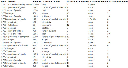
Here are the transactions we generated for this exercise. All we did was to put this table into a spreadsheet, starting in cell A4 with the "details" title.

 

​

 

LOOKUP Table

 

As a matter of interest, we have set up a LOOKUP table to help us to identify the account code numbers. This is not an especially complicated thing to do once you are familiar with LOOKUP functions ... if you download a copy of the spreadsheet that accompanies this page you will see what we have done: click here to get the spreadsheet.

 

Generate a Pivot Table

 

All we do now is to generate a Pivot Table from the transactions, as follows:

 

put the cursor anywhere inside the table of transactions and select

 

Insert tab

Pivot Table

 

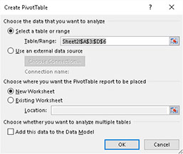
Now follow the dialogue box like this:

 

​

 

Set up your pivot table as you see in the Pivot Table Fields area below

 

Change the layout to the Tabular Style

Switch off sub totals

 

​

 

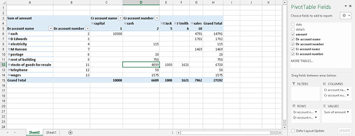
What this matrix does for us is that it adds together all related transactions and tells us the total cash received and paid, the amount spent on postage, the capital investment and so on. We are almost at the stage of having prepared our Trial Balance now!

 

That Pivot Table starts in A1 of the Sheet called pivot and here is the first stage in taking the Trial Balance from it: this table starts in cell I17 of the same sheet. Here is the table and then the formulae that the table uses:

 

First Draft Trial Balance from the Pivot Table

 

Create a new worksheet and call it TB

 

Set up the Trial Balance Template in four columns in this way, starting in cell A1

 

Account Number   Account Name   Dr Amount   Cr Amount

 

The programming of this table uses VLOOKUP(), HLOOKUP() and IFERROR() as well as some minor programming. Look at the screenshot below for full details.

 

​

 

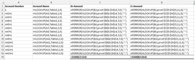
Study the formulas carefully, especially if you have never used these functions before. Notice, I could have used range names in some places but chose not to so read my formulas very carefully.

 

Conclusions

 

That's it! That's all there is to preparing a Trial Balance from a set of bookkeeping transactions. We have used some relatively complex functions and ideas in this discussion but by reviewing this page and Excel's Help pages there is nothing that we cannot do to deal with our transactions!

 

 

Duncan Williamson

9th February 2016